Draw Phase Plane Portrait Mathematica
Return to calculating page for the outset grade APMA0330
Return to computing page for the second course APMA0340
Return to Mathematica tutorial for the start course APMA0330
Return to Mathematica tutorial for the second course APMA0340
Return to the master page for the showtime course APMA0330
Return to the main page for the 2d course APMA0340
Return to Office 2 of the course APMA0340
Introduction to Linear Algebra with Mathematica
Planar Phase Portrait
Consider a systems of linear differential equations with constant coefficients
\begin{equation} \label{EqPhase.1} \dot{\bf ten} = {\bf A}\,{\bf x} , \qquad\mbox{where} \quad \dot{\bf ten} = {\text d}{\bf 10}/{\text d}t , \end{equation}
and A is a square matrix. When matrix A in Eq.\eqref{EqPhase.1} is a 2×2 matrix and x(t) is a 2-dimensional cavalcade vector, this example is chosen planar, and we can have advatange of this to visualize the situation.
Since nosotros know the construction of solutions to Eq.\eqref{EqPhase.1} from its fundamental matrix \( e^{{\bf A}\,t} , \) it is expected that the analysis of solutions nearly the origin is the most fruitful. It is not a surprise that this case requires a special attending.
An autonomous vector differential equation
\begin{equation} \label{EqPhase.2} \dot{\bf 10} = {\bf f} ({\bf ten}) , \qquad\mbox{where} \quad \dot{\bf x} = {\text d}{\bf x}/{\text d}t , \end{equation}
is said to have an equilibrium solution (besides chosen stationary or disquisitional point) x(t) = p if f(p) = 0. The disquisitional bespeak is called isolated if at that place is a neighborhood of the stationary indicate not containing another critical point.
Call up that a neighborhood of a point p is any ready in ℝn that contains an open ball \( \| {\bf ten} - {\bf p} \| = \sqrt{\left( x_1 - p_1 \right)^2 + \cdots +\left( x_n - p_n \right)^ii } < \varepsilon \) centered at p = [p 1, …, p north]T. An equilibrium (too called stationary) solution of the autonomous system \eqref{EqPhase.2} is a point where the derivative of \( {\bf x}(t) \) is zip. An equilibrium solution is a constant solution of the system, and is commonly called a critical point. For a linear arrangement \( \dot{\bf x} = {\bf A}\,{\bf x}, \) an equilibrium solution occurs at each solution of the system (of homogeneous algebraic equations) \( {\bf A}\,{\bf 10} = {\bf 0} . \) Equally we have seen, such a system has exactly one solution, located at the origin, if \( \det{\bf A} \ne 0 .\) If \( \det{\bf A} = 0 , \) then in that location are infinitely many solutions, and the disquisitional signal is not isolated.
Previously, we used a management (or tangent) field to draw the behavior of solutions without actual solving the differential equation. Now we are going to enhance its features past adding arrows to adapt time presence and plot some typical solutions. The authentic tracing of the parametric curves of the solutions is not an easy job without computers. Still, we tin obtain a very reasonable approximation of a trajectory by using the very same thought backside the slope field, namely the tangent line approximation.
The phase portrait of Eq.\eqref{EqPhase.1} or in general, \eqref{EqPhase.two}, is a geometric representation of the trajectories of a dynamical system in the phase plane. The phase portrait contains some typical solution curves along with arrows indicating time variance of solutions (from corresponding direction field) and possible separatrices (if whatsoever).
Recall that a separatrix is the purlieus separating two modes of behaviour in a differential equation and not every dynamoc system has a separatrix. A sketch of a detail solution in the phase plane is called the trajectory or orbit or streamline of the solution. Solutions of Eq.\eqref{EqPhase.i} are plotted as parametric curves (with t every bit the parameter) on the Cartesian airplane tracing the path of each particular solution \( {\bf x} = \left[ x_1 (t) , x_2 (t) \correct]^{\mathrm T} , \ -\infty < t < \infty . \) Similar to a direction field for a single differential equation, a phase portrait is a graphical tool to visualize how the solutions of a given system of differential equations would behave in a neighborhood of the critical point.
We volition classify the disquisitional points of various systems of first order linear differential equations past their stability. Since the general treatment of stability and instability is given in Role Three of this tutorial, it is reasonable to provide its descriptive definition.
A disquisitional point is called an attractor or sink if every solution in a proximity of it moves toward to the stationary point (so it converges to the critical bespeak) as t → +∞. Alternatively, if trajectories most a stationary point leave it equally t → +∞, and then the disquisitional betoken is referred to equally the repeller or source.
Remember that solutions to constant coefficient linear system of differential equations exist for all t ∈ (−∞, ∞). Since the contained variable t is associated with time (which in reality is not invertible), we are mostly interested in understanding the behavior of solutions when t → +∞. However, an attractor becomes a repeller when y'all consider t → −∞ and vice versa. Each gear up of initial conditions is represented past a different curve, or point. They consist of a plot of typical trajectories in the country space. This reveals information such as whether a critical bespeak is an attractor, or a repeller or limit wheel is present for the chosen parameter value.
In add-on, due to the truly ii-dimensional nature of the parametric curves, we will also allocate the type of those critical points based on the behavior of solutions near equilibria (or, rather, by the shape formed by the trajectories near each disquisitional bespeak).
In our report of phase portraits and critical points, we will encounter four types of disquisitional points: nodes, saddle point, spiral, and center. Note that this is typical only for two-dimensional problems. Additionally, these disquisitional points are based on the eigenvalues and eigenvectors of the abiding coefficient linear system of differential equations. The table below emphasizes the relationship between the stability and type of critical point based on the eigenvalues.
If a square matrix is singular, then at least one of its eigenvalues is cypher. In this case, the origin is not an isolated critical indicate and there is a line of stationary points. This line is an eigenspace corresponding to the nothing eigenvalue and it is also a separatrix in the phase portrait.
Case 1: Consider the 2×2 matrix
\[ {\bf A} = \begin{bmatrix} 1&2 \\ ii& 4 \end{bmatrix} . \]
Information technology has two eigenvalues
A = {{1, 2}, {2, 4}}
Eigenvalues[A]
{5, 0}
And so nosotros find the corresponding eigenvectors:
Eigenvectors[A]
{{1, two}, {-ii, 1}}
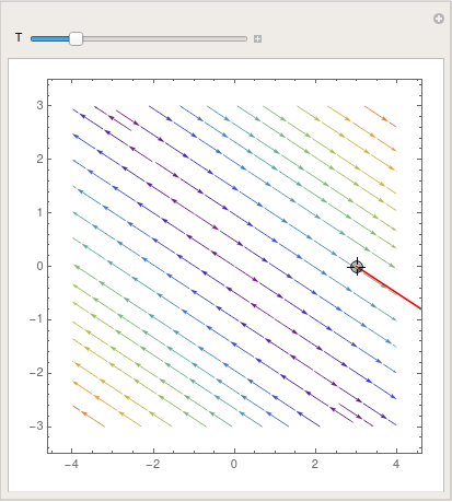
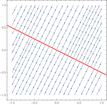 | So we know that the eigenvalue λ = 0 has a corresponding eigenvector [−two, 1]. Then we plot the direction field along with the separatrix respective to the eigenspace of λ = 0. sp = StreamPlot[{x + 2*y, 2*x + four*y}, {10, -i, one}, {y, -1, 1}]; | |
| Separatrix is an case of non-isolated equilibria. | Mathematica code |
■
Isolated Equilibria
As a rule, we will merely consider systems of linear differential equations whose coefficient matrix A has a nonzero determinant.
In two-dimensional space, it is possible to completely classify the critical points of various systems of first lodge linear differential equations past their stability. In addition, due to the truly two-dimensional nature of the parametric curves, nosotros will also classify the type of those critical points past their shapes (or, rather, by the shape formed past the trajectories near each critical betoken). Their classification is based on eigenvalues of the coefficient matrix. Therefore, we consider unlike cases.
There are four types of critical points. To characterize them, it is convenient to use polar coordinates. Suppose that the solution curve of the autonomous planar differential equation dx/dt = f(x) can be written equally 10 = x(t), y = y(t), where x = [x(t), y(t)]T is a two-dimensional column vector. So in polar coordinates, their trajectory can exist written as
\begin{equation} \label{EqPhase.3} r = \rho (t) \ge 0, \qquad \theta = \omega (t) , \end{equation}
with ten(t) = ρ(t) cosω(t), y(t) = ρ(t) sinω(t). For matrix \( {\bf A} = \begin{bmatrix} a & b \\ c& d \cease{bmatrix} , \) the polar variables satisfy the equations:
\begin{equation} \label{EqPhase.4} \dot{r} = r \left[ a\,\cos^2 \theta + \left( b+c \right) \cos\theta\,\sin\theta + d\,\sin^2 \theta \right] , \qquad \dot{\theta} = c\,\cos^two \theta + \left( d-a \right) \cos\theta\,\sin \theta -b\,\sin^2 \theta . \end{equation}
A critical betoken (0,0) of the constant coefficient democratic equation \eqref{EqPhase.1} is said to be a node if \( \lim_{t\to +\infty} \left\vert \omega (t) \correct\vert = \) constant or \( \lim_{t\to -\infty} \left\vert \omega (t) \right\vert = \) constant, when ten(t) belongs to some neighborhood of the critical point. In the old case, the critical betoken is called nodal sink, and in latter, it is a nodal source.
Nodes are disquisitional points with the holding that a trajectories arrive or depart from the disquisitional point along some directory. In plough, there are known of three types of nodes:
- proper node or star when every semi-line from the critical point is a tangent to some orbit;
- improper node when in that location are at most two directions forth which trajectories arroyo the disquisitional betoken;
- degenerate node when there is only one management along which orbits approach the disquisitional indicate.
An equilibrium solution of an autonomous system of differential equations \( \dot{\bf ten} = {\bf f}\left( {\bf x}\right) \) is chosen a node if nearby trajectories arroyo it or depart from the critical bespeak along some definite direction (semi-straight line). Correspondingly, the critical point is referred to equally nodal sink or nodal source, depending whether trajectories approach the stationary point or depart from it as t → +∞.
The trajectories that are the eigenvectors move in straight lines. The residuum of the trajectories motion, initially when near the critical point, roughly in the same direction as the eigenvector of the eigenvalue with the smaller absolute value. Then, farther away, they would bend toward the management of the eigenvector of the eigenvalue with the larger absolute value.
For constant coefficient linear differential equations, classification of critical points can be performed based on eigenvalues of the corresponding abiding matrix.
Case 1: Diagonal existent-valued matrix with the same entries and of the same sign. A proper node can exist observed only when the matrix of the system is a abiding existent multiple of the diagonal matrix:
\[ \alpha \, \begin{bmatrix} 1&0 \\ 0&1 \end{bmatrix} = \brainstorm{bmatrix} \alpha &0 \\ 0&\alpha \end{bmatrix} \quad \mbox{ where } \blastoff \quad \mbox{is an arbitrary nonzero constant} . \]
In this case, the organisation is uncoupled and each equation tin can be solved separately. Numbers on the diagonal are eigenvalues of the matrix. See the following instance. And so the general solution is
\[ {\bf y}(t) = \brainstorm{bmatrix} y_1 (t) \\ y_2 (t) \end{bmatrix} = c_1 \begin{bmatrix} \eleven \\ 0 \end{bmatrix} e^{\lambda\,t} + c_2 \begin{bmatrix} 0 \\ \eta \stop{bmatrix} east^{\lambda\,t} , \]
with arbitrary constants c ane and c 2.
Example 2: Consider the following 2×2 matrices
\[ {\bf A}_1 = \begin{bmatrix} ane&0 \\ 0& ane \end{bmatrix} , \qquad {\bf A}_2 = \brainstorm{bmatrix} -ane&\phantom{-}0 \\ \phantom{-}0& -1 \cease{bmatrix} . \]
Upon plotting the respective phase portraits, we run into that matrix A ane generate proper nodal source at the origin, whereas matrix A 2 corresponds to proper nodal sink.
StreamPlot[{10, y}, {x, -1, 1}, {y, -1, 1}, ClippingStyle -> {Blue, Scarlet}]
VectorPlot[{x, two*y}, {x, -1, ane}, {y, -1, 1}, PlotTheme -> "Scientific"]
StreamPlot[{-x, -y}, {x, -ane, ane}, {y, -1, 1}, StreamPoints -> xxx]
VectorPlot[{-10, -2*y}, {x, -1, 1}, {y, -1, 1}, PlotTheme -> "Web"]
■
Case two: Distinct existent eigenvalues of the same sign. Then the general solution of the linear organisation \( \dot{\bf x} = {\bf A}\,{\bf x}, \) is
\[ {\bf 10} (t) = c_1 \,{\bf \xi} \, e^{\lambda_1 t} + c_2 \,{\bf \eta} \, due east^{\lambda_2 t} , \]
where \( \lambda_1 \) and \( \lambda_2 \) are distinct real eigenvalues, \( {\bf \xi} \) and \( {\bf \eta} \) are corresponding eigenvectors, and \( c_1 , c_2 \) are arbitrary existent constants.
When eigenvalues λ1 and λii are both positive, or are both negative, the stage portrait shows trajectories either moving away from the disquisitional point toways infinity (for positive eigenvalues), or moving directly towards and converging to the critical point (for negative eigenvalues). The trajectories that are the eigenvectors motion in straight lines. The residue of the trajectories move, initially when near the critical point, roughly in the same direction as the eigenvector of the eigenvalue with the smaller accented value. And then, farther away, they would bend toward the direction of the eigenvector of the eigenvalue with the larger absolute value. This type of disquisitional point is called a node. It is asymptotically stable if eigenvalues are both negative, unstable if eigenvalues are both positive.
Stability: It is unstable if both eigenvalues are positive; asymptotically stable if they are both negative.
Example three: We start with the diagonal matrix and corresponding democratic differential equation
\[ {\bf B} = \begin{bmatrix} i&0 \\ 0&2 \end{bmatrix} , \qquad \frac{{\text d}{\bf y}}{{\text d}t} = {\bf B} \,{\bf y}(t) . \]
So the given arrangement is decoupled
\[ \dot{x} = x , \qquad \dot{y} = 2\,y , \]
with the full general solution
\[ {\bf y}(t) = \begin{bmatrix} x(t) \\ y(t) \end{bmatrix} = c_1 \begin{bmatrix} one \\ 0 \end{bmatrix} eastward^{t} + c_2 \brainstorm{bmatrix} 0 \\ ane \end{bmatrix} east^{2t} . \]
Hither, c ane and c ii are capricious constants. We can notice the explicit solution from the equation
\[ \frac{{\text d}y}{{\text d}ten} = \frac{\dot{y}}{\dot{10}} = \frac{2y}{x} \qquad \Longrightarrow \qquad y = x^two . \]
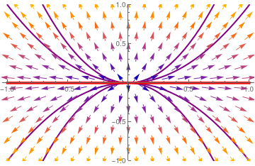 | We plot the direction field along with some trajectories and separatrix y = 0. Another eigenspace x = 0 (vertical line) is not actually a separatrix, and it is non shown. vp = VectorPlot[{10, two*y}, {10, -one, 1}, {y, -1, one}, PlotTheme -> "Scientific"]; Mathematica code. | |
| Separatrix y = 0 (in red) and phase portrait for matrix B. The origin is a nodal source---repeller. |
For another diagonal matrix
\[ {\bf B}_2 = \begin{bmatrix} -1&\phantom{-}0 \\ \phantom{-}0&-iii \end{bmatrix} , \qquad \frac{{\text d}{\bf y}}{{\text d}t} = {\bf B}_2 \,{\bf y}(t) . \]
nosotros take a similar phase portrait, only the origin becomes nodal sink.
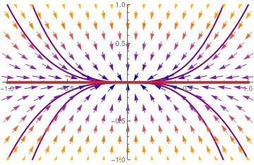 | Upon separation of variables, nosotros obtain its general solution \[ \frac{{\text d}y}{{\text d}ten} = \frac{\dot{y}}{\dot{x}} = \frac{-3y}{-x} \qquad \Longrightarrow \qquad y = x^iii . \] We plot the direction field along with some trajectories and separatrix y = 0 vp = VectorPlot[{-10, -3*y}, {10, -one, i}, {y, -i, i}, PlotTheme -> "Scientific"]; | |
| Separatrix y = 0 (in red) and phase portrait for matrix B 2. The origin is a nodal sink (attractor). | Mathematica code |
■
An example of a stable node is provided by the overdamped oscillator: \( \ddot{x} + 3\dot{10} + x = 0 . \)
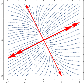
Example 4: Consider ii matrices
\[ {\bf A}_1 = \begin{bmatrix} -5&2 \\ -4&1 \finish{bmatrix} , \qquad {\bf A}_2 = \begin{bmatrix} 2&i \\ 1&two \end{bmatrix} \]
A1 = {{-5, 2}, {-4, 1}}
Eigenvalues[A1]
{-three, -one}
This tells us that the origin is the attractor because both eigenvalues are real negative numbers.
Eigenvectors[A1]
{{one, i}, {1, ii}}
And so we know that separatrix is going along each eigenvector corresponding to distinct eigenvalues. We plot the respective eigenlines; one of them corresponding to the largest absolute value (λ = −3) is indicated past double arrow and another eigenline (λ = −one) is labeled by a single arrow.
arr1 = Graphics[{Red, Thick, Arrowheads[0.06], Arrow[{{1, i}, {0, 0}}]}];
arr1a = Graphics[{Red, Thick, Arrowheads[0.06], Arrow[{{1, i}, {0.1, 0.1}}]}];
arr2 = Graphics[{Regal, Thick, Arrowheads[0.06], Pointer[0.five*{{1, 2}, {0.2, 0.4}}]}];
arr4 = Graphics[{Imperial, Thick, Arrowheads[0.06], Arrow[0.five*{{-1, -2}, {-0.2, -0.four}}]}];
arr3 = Graphics[{Cerise, Thick, Arrowheads[0.06], Arrow[{{-one, -one}, {0, 0}}]}];
arr3a = Graphics[{Red, Thick, Arrowheads[0.06], Pointer[{{-1, -1}, {-0.one, -0.1}}]}];
sp = StreamPlot[{-5*x + 2*y, -4*x + y}, {10, -1, 1}, {y, -ane, 1}, PlotTheme -> "Scientific", StreamStyle -> Blue];
Show[arr1, arr1a, arr2, arr3, arr3a, arr4, sp]
Now nosotros perform a similar job with another matrix A two.
A2 = {{2, ane}, {ane, 2}}
Eigenvalues[A2]
{iii, i}
This tells us that the origin is a repeller because both eigenvalues are real positive numbers.
Eigenvectors[A2]
{{1, one}, {-1, ane}}
vp = VectorPlot[{ii*x + y, 10 + two*y}, {ten, -1, 1}, {y, -1, i}, StreamStyle -> Blue];
arr1 = Graphics[{Red, Thick, Arrowheads[0.06], Pointer[{{0, 0}, {one, 1}}]}];
arr1a = Graphics[{Red, Thick, Arrowheads[0.06], Pointer[{{0, 0}, {0.9, 0.9}}]}];
arr2 = Graphics[{Orange, Thick, Arrowheads[0.06], Arrow[{{0, 0}, {-1, 1}}]}];
arr4 = Graphics[{Orange, Thick, Arrowheads[0.06], Pointer[{{0, 0}, {1, -i}}]}];
arr3 = Graphics[{Red, Thick, Arrowheads[0.06], Arrow[{{0, 0}, {-1, -1}}]}];
arr3a = Graphics[{Crimson, Thick, Arrowheads[0.06], Pointer[{{0, 0}, {-0.nine, -0.9}}]}];
Show[arr1, arr1a, arr2, arr3, arr3a, arr4, vp]
The graphs below prove phase portrait around the critical indicate (origin) along with separatricies that go along eigenlines (generated by eigenvectors). The eigenline corresponding to the dominant eigenvalue (having largest absolute value) is shown with double arrow and blood-red color.
■
Instance 3: Repeated real eigenvalue with ane eigenvector. If a square 2×2 matrix is not diagonal and has a defective (repeated) eigenvalue, then the matrix has only one eigenvector. It is not diagonalizable and its general solution is of the class
\[ {\bf ten} (t) = e^{{\bf A}t} {\bf c} = c_1 \,{\bf \xi} \, east^{\lambda\, t} + c_2 \,east^{\lambda\, t} \left( t\,{\bf \xi} + {\bf \eta} \correct) , \]
where ξ is the eigenvector and η is so called the generalized eigenvector. The original is the degenerate node, either attractor if its eigenvalue is negative, or repeller if its eigenvalue is positive. The trajectories either all diverge away from the critical point towards infinity (when eigenvalue λ > 0) or all converge towards the disquisitional signal (when eigenvalue λ < 0). This type of critical point is called an improper node. It is asymptotically stable if \( \lambda <0 ,\) unstable if \( \lambda >0 .\) The phase portrait is presented in the following example.
Example five: Consider two matrices
\[ {\bf A}_3 = \begin{bmatrix} 5&-three \\ 3& -1 \cease{bmatrix} , \qquad {\bf A}_4 = \begin{bmatrix} -v&-3 \\ \phantom{-}3&\phantom{-}1 \cease{bmatrix} . \]
Using Mathematica, we make up one's mind that matrix A 3 has one defective eigenvalue λ = 2; this tells united states of america that the origin is the repeller.
A3 = {{5, -3}, {three, -ane}};
Eigenvalues[A3]
{2, 2}
Eigenvectors[A3]
{{one, ane}, {0, 0}}
We plot the direction field and the separatrix (in red) that is spanned on the eigenvectors.
vp = VectorPlot[{5*10 - 3*y, three*x - y}, {x, -one, 1}, {y, -ane, 1}, StreamStyle -> Blue];
line = Graphics[{Red, Thick, Line[{{-1, -i}, {one, 1}}]}];
Evidence[line, vp]
Then we repeat the same job for matrix A 4.
A4 = {{-five, -3}, {three, 1}};
Eigenvalues[A3]
{-2, -2}
Eigenvectors[A4]
{{-one, 1}, {0, 0}}
sp = StreamPlot[{-5*x - 3*y, 3*x + y}, {10, -i, i}, {y, -one, i}, StreamStyle -> Bluish];
line = Graphics[{Red, Thickness[0.01], Line[{{-1, 1}, {ane, -1}}]}];
Bear witness[line, sp]
■
A critical point (0,0) of the abiding coefficient autonomous equation \eqref{EqPhase.1} is said to be a saddle betoken if in that location are two trajectories approaching the origin along opposite directions, and all other orbits shut to either of them and to (0,0) tend abroad from them as t becomes space.
Case 4: Distinct real eigenvalues are of reverse signs. In this type of stage portrait, the trajectories given by the eigenvectors of the negative eigenvalue initially beginning at infinity before moving towards and eventually converging at the critical point. The trajectories that represent the eigenvectors of the positive eigenvalue movement in exactly the opposite fashion: starting at the critical point earlier diverging to infinity. Every other trajectory starts at infinity, moves toward but never converges to the disquisitional point, and then changes direction and moves back towards infinity. All the while it would roughly follow the 2 sets of eigenvectors. This type of critical point is chosen a saddle point. It is ever unstable.
Stability: It is always unstable.
Example half-dozen: Consider a system of ordinary differential equations
\[ \frac{{\text d}}{{\text d} t} \begin{bmatrix} x_1 \\ x_2 \end{bmatrix} = \begin{bmatrix} 1&two \\ 2&1 \end{bmatrix} \, \begin{bmatrix} x_1 \\ x_2 \end{bmatrix} . \]
We can enter this equation into Mathematica either as a vector
f[x_, y_] = {x + two*y, 2*10 + y}; Print["X' = ", MatrixForm[f[x, y]]]
\( Ten' = \begin{pmatrix} x+ii\,y\\ 2\,10 +y \end{pmatrix} \)
or as two equations
Print["10' = ", f[x, y][[1]], ", y' = ", f[x, y][[ii]]]
\( 10' = x + two\,y, \quad y' = 2\,x + y \)
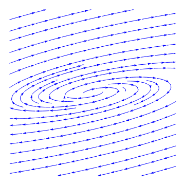
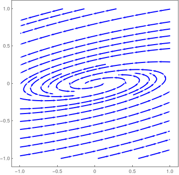
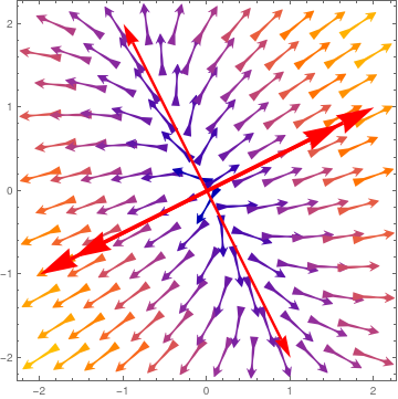
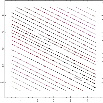
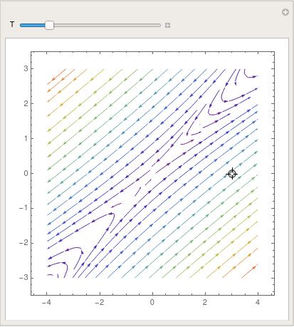
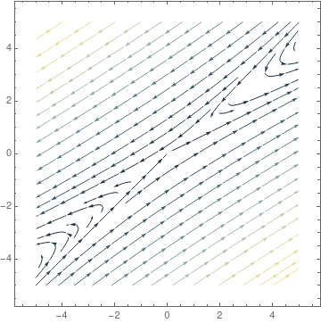
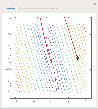
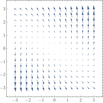
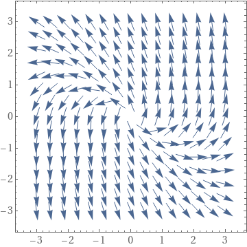
The coefficient matrix \( {\bf A} = \begin{bmatrix} 1&2 \\ 2&one \end{bmatrix} \) has 2 distinct existent eigenvalues \( \lambda_1 =iii \) and \( \lambda_2 =-one . \) Therefore, the critical point, which is the origin, is a saddle point, unstable. Nosotros plot the corresponding stage portrait using the following codes. Mathematica provides us at least ii options: either StreamPlot or VectorPlot (for the latter nosotros requite two versions without normalization and with it).
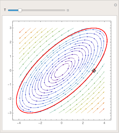
splot = StreamPlot[{10 + two*y, two*x + y}, {x, -4, 4}, {y, -3, 3}, StreamColorFunction -> "Rainbow"];
Manipulate[ Show[splot, ParametricPlot[ Evaluate[ First[{x[t], y[t]} /.
NDSolve[{x'[t] == 10[t] + 2*y[t], y'[t] == two*x[t] + y[t], Thread[{10[0], y[0]} == signal]}, {x, y}, {t, 0, T}]]], {t, 0, T}, PlotStyle -> Cerise]], {{T, xx}, ane, 100}, {{signal, {3, 0}}, Locator}, SaveDefinitions -> True]
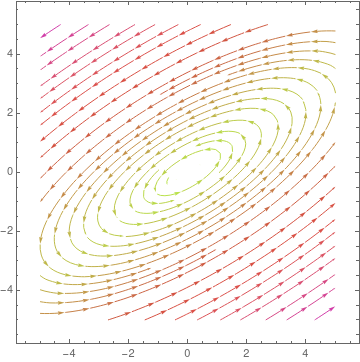
and the phase portrait with VectorPlot
Bear witness[VectorPlot[f[ten, y], {ten, -4, 4}, {y, -four, iv}], Frame -> True, BaseStyle -> {FontFamily -> "Times", FontSize -> 14}]
Evidence[VectorPlot[f[x, y]/Norm[f[x, y]], {x, -4, iv}, {y, -four, 4}], Frame -> Truthful, BaseStyle -> {FontFamily -> "Times", FontSize -> 14}]
| StreamPlot | VectorPlot | VectorPlot with normalization |
|---|---|---|
 | 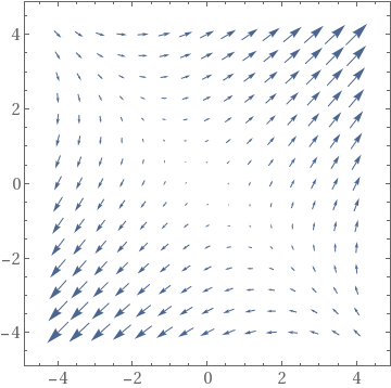 | 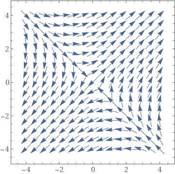 |
Information technology is clear that the origin is an unstable equilibrium solution. ■
A disquisitional point (0,0) of the constant coefficient autonomous equation \eqref{EqPhase.1} is said to be a screw signal if the following 3 conditions concur for all orbits in some neighbohood of the origin.
- all trajectories are defined on t 0 < t < ∞ or −∞ < t < t 0 for some t 0;
- \( \lim_{t\to +\infty} r (t) = 0 \) or \( \lim_{t\to -\infty} r (t) = 0 . \)
- \( \lim_{t\to +\infty} \left\vert \omega (t) \right\vert = \infty \) or \( \lim_{t\to -\infty} \left\vert \omega (t) \correct\vert = \infty . \)
Case 5: Complex conjugate eigenvalues. When the real office of eigenvalues is nonzero, the trajectories nonetheless retain the elliptical traces. Nonetheless, with each revolution, their distances from the critical point grow/decay exponentially according to the term \( e^{\Re\lambda\,t} , \) where \( \Re\lambda \) is the real part of the complex λ, the eigenvalue. Therefore, the phase portrait shows trajectories that spiral away from the disquisitional point toways infinity (when \( \Re\lambda > 0 \) ), or trajectories that screw toward, and converge to the disquisitional bespeak (when \( \Re\lambda < 0 \) ). This blazon of critical point is called a spiral point. It is asymptotically stable if \( \Re\lambda < 0 ,\) it is unstable if \( \Re\lambda > 0 . \)
An case of a stable spiral is provided by the underdamped oscillator: \( \ddot{x} + \dot{x} + ten = 0 . \)
Example 7: Consider ii matrices
\[ {\bf A}_5 = \begin{bmatrix} -1&xiii \\ -1& \phantom{1}3 \stop{bmatrix} , \qquad {\bf A}_6 = \begin{bmatrix} -3&thirteen \\ -1&\phantom{3}1 \end{bmatrix} . \]
The eigenvalues of both matrices are complex conjugate numbers:
A5 = {{-i, thirteen}, {-1, iii}}; Eigenvalues[A5]
{ane + 3 I, 1 - iii I}
and
A6 = {{-iii, 13}, {-1, one}}; Eigenvalues[A6]
{-1 + 3 I, -1 - 3 I}
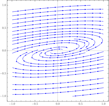 | We plot the management field in a neighborhood of the asymptotically stable stationary point. Notation that trajectories arroyo the origin in clockwise direction. StreamPlot[{-3*x + 13*y, -x + y}, {x, -1, one}, {y, -i, 1}, PlotTheme -> "Scientific", StreamStyle -> Blue, PerformanceGoal -> "Quality", StreamPoints -> 25] | |
| Screw critical point for matrix A half-dozen. | Mathematica lawmaking |
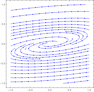 | Nosotros plot the direction field in a neighborhood of the asymptotically stable stationary point for matrix −A six. Note that trajectories approach the origin in counterclockwise management. StreamPlot[{iii*x - xiii*y, x - y}, {x, -ane, 1}, {y, -1, i}, PlotTheme -> "Detailed", StreamStyle -> Blue, PerformanceGoal -> "Quality", StreamPoints -> 25] | |
| Spiral asymptotically stable critical point for matrix −A 6. | Mathematica lawmaking |
Now we do a similar job for matrix A v that has unstable critical signal at the origin.
 | We plot the direction field in a neighborhood of the ustable stationary indicate. Note that trajectories depart from the origin in clockwise direction. StreamPlot[{-x + 13*y, -x + 3*y}, {10, -1, one}, {y, -ane, i}, PlotTheme -> "Minimal", StreamStyle -> Blueish, PerformanceGoal -> "Quality", StreamPoints -> 25] | |
| Spiral unstable critical betoken for matrix A 5. | Mathematica code |
 | Nosotros plot the direction field in a neighborhood of the unstable stationary point for matrix −A 5. Note that trajectories depart from the origin in counterclockwise direction. StreamPlot[{ten - 13*y, ten - 3*y}, {x, -1, 1}, {y, -one, 1}, PlotTheme -> "Web", StreamStyle -> Blue, PerformanceGoal -> "Quality", StreamPoints -> 25] | |
| Screw unstable critical point for matrix −A 5. | Mathematica code |
■
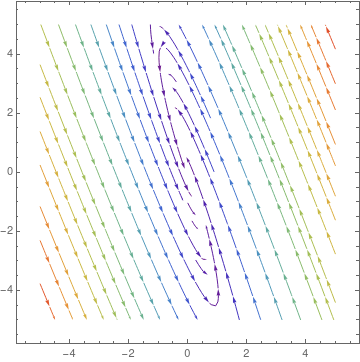
A critical point (0,0) of the constant coefficient autonomous equation \eqref{EqPhase.1} is said to be a heart if there exists a neighborhood containing countably many closed trajectories, each containing the origin and diameters tend to nothing.
Case half dozen: Two pure complex conjugate eigenvalues. When the real office of the eigenvalues is nix, the trajectories neither converge to the disquisitional point nor move toways infinitey. Rather, they stay in constant, elliptical (or, rarely, circular) orbits. This type of disquisitional point is chosen a center. Information technology has a unique stability nomenclature shared past no other: stable (or neutrally stable).
An example of a middle is provided by the uncomplicated harmonic oscillator: \( \ddot{x} + x = 0 . \)
Example 8: Consider the system of differential equations
\[ \frac{{\text d}{\bf x}}{{\text d}t} \equiv \frac{\text d}{{\text d}t} \begin{bmatrix} 10(t) \\ y(t) \end{bmatrix} = \brainstorm{bmatrix} 10-y \\ 5x-y \terminate{bmatrix} . \]
The corresponding matrix
\[ {\bf A} = \brainstorm{bmatrix} 1&-1 \\ 5&-1 \end{bmatrix} \]
has two complex cohabit pure imaginary eigenvalues
B = {{one, -1}, {v, -1}}; Eigenvalues[B]
{two I, -2 I}
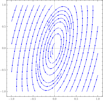 | Nosotros plot the direction field. StreamPlot[{x -y, 5*10 - y}, {x, -one, i}, {y, -1, i}, PlotTheme -> "Scientific", StreamStyle -> Bluish, PerformanceGoal -> "Quality", StreamPoints -> 25] | |
| Center disquisitional point. | Mathematica code |
■
| Eigenvalues | Condition | Blazon of Critical Signal | Stability |
|---|---|---|---|
| λi > λtwo > 0 | tr(A) > 0 and tr²(A) > 4 det(A), det(A) > 0 | Nodal source (node) | Unstable |
| λi < λ2 < 0 | tr(A) < 0 and tr²(A) > iv det(A), det(A) > 0 | Nodal sink (node) | Asymptotically stable |
| λ1 < 0 < λ2 | detA < 0 | Saddle betoken | Unstable |
| λ1 = λtwo > 0 diagonal matrix | A = 1000I with k>0 | Proper node (star) | Unstable |
| λ1 = λ2 < 0 diagonal matrix | A = mI with thou<0 | Proper node (star) | Asymptotically stable |
| λ1 = λ2 > 0 missing eigenvector | A = k 1I + k 2I with k>0 | Improper/degenerate node | Unstable |
| λ1 = λ2 < 0 missing eigenvalue | A = k aneI + k iiI with m<0 | Improper/degenerate node | Asymptotically stable |
| λ = α ± jβ, α > 0 | tr(A) > 0 and tr²(A) < 4 det(A) | Screw point | Unstable |
| λ = α ± jβ, α < 0 | tr(A) < 0 and tr²(A) < four det(A) | Screw point | Asymptotically stable |
| λ = ± jβ | tr(A) = 0 and tr²(A) < 4 det(A) | Center | Stable |
Mathematica plots stage portraits
Mathematica gives several options to plot phase portraits for planar systems of differential equations. We testify them by examples. Matrix
\[ \brainstorm{bmatrix} 13&4 \\ four&7 \end{bmatrix} \]
has two positive distinct eigenvalues
c = {{13, 4}, {4, 7}};
Eigenvalues[c]
{15, 5}
Eigenvectors[c]
{{2, 1}, {-ane, 2}}
 | Then we plot direction field and two separatrices using StreamPlot ar1 = Graphics[{Carmine, Thickness[0.01], Arrowheads[0.1], Arrow[{{0, 0}, {two, ane}}]}]; | |
| Nodal repeller and two separatreces. | Mathematica code |
 | Then we plot the management field with VectorPlot command. As usual, the dominated eigenspace is identified with double arrow. ar1 = Graphics[{Red, Thickness[0.01], Arrowheads[0.i], Arrow[{{0, 0}, {2, 1}}]}]; | |
| Ii Separatrices dissever the phase plane into four parts. | Mathematica code |
We can take advantage of the Manipulate command that allows one to change
(in our example) the initial point along with the direction field:
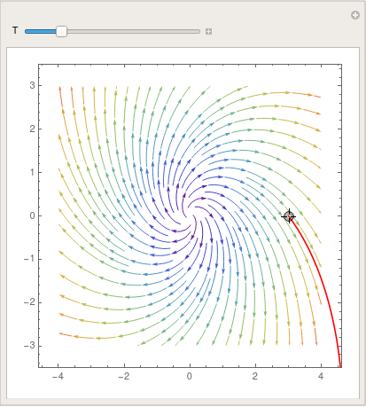 | parta = StreamPlot[{x + y, y - x}, {x, -four, 4}, {y, -3, 3}, | |
| Demonstration of Manipulate command. | Mathematica lawmaking |
To save the image, use Mathematica command Consign:
Export["foo.gif",%]
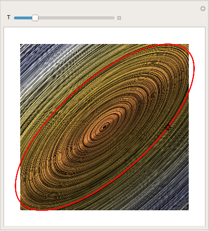
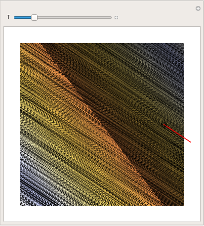
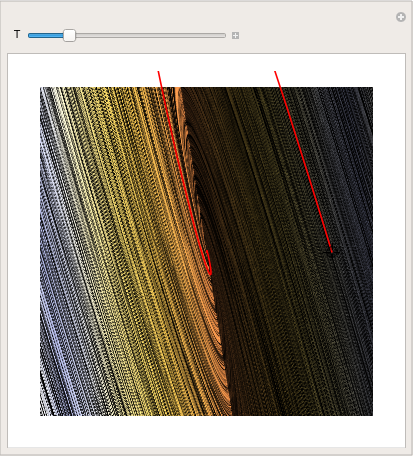
You can even make a absurd pic by using LineIntegralConvolutionPlot:
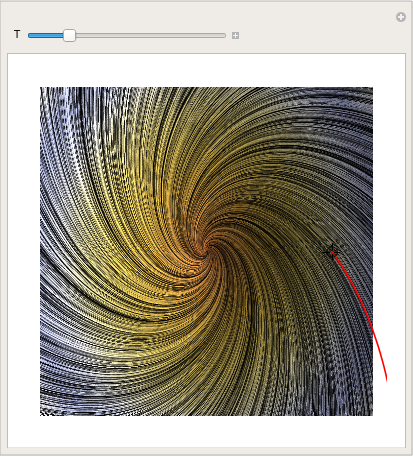 | parta = LineIntegralConvolutionPlot[{{ten + y, y - x}, {"noise", thou, | |
| Sit-in of LineIntegralConvolutionPlot command. | Mathematica code |
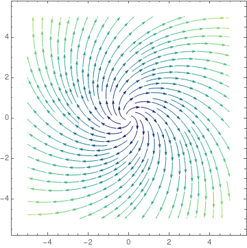
To put iii colors into the plot, ane may use
StreamPlot[{ten + y, y - 10}, {10, -5, 5}, {y, -5, five}, StreamColorFunction -> "BlueGreenYellow"]
partb = StreamPlot[{10 - 2*y, x - y}, {ten, -four, 4}, {y, -3, 3},
StreamColorFunction -> "Rainbow"];
Manipulate[
Evidence[partb,
ParametricPlot[
Evaluate[
First[{x[t], y[t]} /.
NDSolve[{x'[t] == x[t] - 2*y[t], y'[t] == -y[t] + x[t],
Thread[{ten[0], y[0]} == signal]}, {x, y}, {t, 0, T}]]], {t, 0,
T}, PlotStyle -> Cherry-red]], {{T, 20}, 1, 100}, {{indicate, {iii, 0}},
Locator}, SaveDefinitions -> True]
To relieve the image as gif-file, type:
Consign["foo.gif",%]
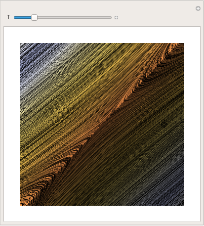
partb = LineIntegralConvolutionPlot[{{x - 2*y, x - y}, {"noise", 1000, yard}}, {x, -4,
four}, {y, -iii, three}, ColorFunction -> "BeachColors",
LightingAngle -> 0, LineIntegralConvolutionScale -> 3,
Frame -> Imitation];
Dispense[
Show[partb,
ParametricPlot[
Evaluate[
Showtime[{x[t], y[t]} /.
NDSolve[{ten'[t] == ten[t] - two*y[t], y'[t] == -y[t] + 10[t],
Thread[{x[0], y[0]} == point]}, {x, y}, {t, 0, T}]]], {t, 0,
T}, PlotStyle -> Red]], {{T, xx}, ane, 100}, {{point, {3, 0}},
Locator}, SaveDefinitions -> True]
Export["foo.gif",%]
matrixb = StreamPlot[{ten - 2*y, x - y}, {x, -5, 5}, {y, -5, 5}, StreamColorFunction -> "NeonColors"]
partc = StreamPlot[{2*x + 2*y, -y - x}, {x, -4, 4}, {y, -3, 3},
StreamColorFunction -> "Rainbow"];
Manipulate[
Testify[partc,
ParametricPlot[
Evaluate[
First[{10[t], y[t]} /.
NDSolve[{ten'[t] == ii*ten[t] + 2*y[t], y'[t] == -y[t] - x[t],
Thread[{x[0], y[0]} == point]}, {10, y}, {t, 0, T}]]], {t, 0,
T}, PlotStyle -> Red]], {{T, 20}, 1, 100}, {{point, {3, 0}},
Locator}, SaveDefinitions -> True]
Consign["foo.gif",%]
partc = LineIntegralConvolutionPlot[{{2*ten + ii*y, -y - 10}, {"racket", 1000,
1000}}, {x, -4, 4}, {y, -3, 3}, ColorFunction -> "BeachColors",
LightingAngle -> 0, LineIntegralConvolutionScale -> 3,
Frame -> Fake];
Dispense[
Show[partc,
ParametricPlot[
Evaluate[
Starting time[{10[t], y[t]} /.
NDSolve[{x'[t] == 2*x[t] + 2*y[t], y'[t] == -y[t] - x[t],
Thread[{x[0], y[0]} == signal]}, {x, y}, {t, 0, T}]]], {t, 0,
T}, PlotStyle -> Red]], {{T, 20}, 1, 100}, {{signal, {three, 0}},
Locator}, SaveDefinitions -> Truthful]
matrixc =
StreamPlot[{2*10 + 2*y, -10 - y}, {x, -v, 5}, {y, -v, v},
StreamColorFunction -> "PlumColors"]
partd = StreamPlot[{5*10 - half dozen*y, 3*x - 4*y}, {x, -4, 4}, {y, -3, 3},
StreamColorFunction -> "Rainbow"];
Manipulate[
Prove[partd,
ParametricPlot[
Evaluate[
Get-go[{10[t], y[t]} /.
NDSolve[{x'[t] == five*10[t] - vi*y[t], y'[t] == three*ten[t] - 4*y[t],
Thread[{x[0], y[0]} == point]}, {x, y}, {t, 0, T}]]], {t, 0,
T}, PlotStyle -> Red]], {{T, 20}, 1, 100}, {{indicate, {3, 0}},
Locator}, SaveDefinitions -> True]
partd = LineIntegralConvolutionPlot[{{5*x - 6*y, 3*10 - 4*y}, {"noise", chiliad,
1000}}, {x, -4, 4}, {y, -3, 3}, ColorFunction -> "BeachColors",
LightingAngle -> 0, LineIntegralConvolutionScale -> 3,
Frame -> Imitation];
Manipulate[
Show[partd,
ParametricPlot[
Evaluate[
First[{x[t], y[t]} /.
NDSolve[{x'[t] == five*x[t] - half-dozen*y[t], y'[t] == 3*x[t] - four*y[t],
Thread[{x[0], y[0]} == point]}, {x, y}, {t, 0, T}]]], {t, 0,
T}, PlotStyle -> Reddish]], {{T, xx}, 1, 100}, {{indicate, {3, 0}},
Locator}, SaveDefinitions -> True]
matrixd =
StreamPlot[{5*x - 6*y, iii*10 - 4*y}, {10, -v, v}, {y, -5, 5},
StreamColorFunction -> "StarryNightColors"]
parte = StreamPlot[{-4*x - y, ii*y + 10*ten}, {x, -four, 4}, {y, -3, 3},
StreamColorFunction -> "Rainbow"];
Dispense[
Prove[parte,
ParametricPlot[
Evaluate[
Commencement[{x[t], y[t]} /.
NDSolve[{x'[t] == -four*x[t] - y[t], y'[t] == 2*y[t] + ten*x[t],
Thread[{x[0], y[0]} == signal]}, {x, y}, {t, 0, T}]]], {t, 0,
T}, PlotStyle -> Blood-red]], {{T, 20}, i, 100}, {{point, {three, 0}},
Locator}, SaveDefinitions -> True]
parte = LineIntegralConvolutionPlot[{{-4*x - 1*y, x*x + 2*y}, {"racket", thou,
1000}}, {x, -four, iv}, {y, -iii, 3}, ColorFunction -> "BeachColors",
LightingAngle -> 0, LineIntegralConvolutionScale -> three,
Frame -> Imitation];
Manipulate[
Evidence[parte,
ParametricPlot[
Evaluate[
First[{x[t], y[t]} /.
NDSolve[{x'[t] == -4*x[t] - one*y[t], y'[t] == 10*ten[t] + 2*y[t],
Thread[{ten[0], y[0]} == signal]}, {ten, y}, {t, 0, T}]]], {t, 0,
T}, PlotStyle -> Crimson]], {{T, 20}, ane, 100}, {{signal, {three, 0}},
Locator}, SaveDefinitions -> True]
matrixe = StreamPlot[{-4*x - y, 10*x + two*y}, {10, -5, 5}, {y, -5, 5}, StreamColorFunction -> "Rainbow"]
There is another way to visualize solutions to vector differential eastward quation---utilize VectorPlot :
A={{1,-2},{iii,5}};
Show[VectorPlot[A.{x, y}, {x, -3, 3}, {y, -3, 3}], Frame -> True,
BaseStyle -> {FontFamily -> "Times", FontSize -> 14}]
If one wants to run into equal size arrows, type:
Prove[VectorPlot[
A.{x, y}/(10^-8 + Norm[A.{x, y}]), {ten, -iii, 3}, {y, -three, 3}],
Frame -> True, BaseStyle -> {FontFamily -> "Times", FontSize -> 14}]
If you have a list of square matrices, and yous desire to determine stability of the origin for each matrix, it makes sense to organize it is a loop. For case,
A1 = {{2, 4}, {7, 5}};
A2 = {{-1, ii}, {-5, 5}};
A3 = {{1, -vi}, {half-dozen, ane}};
A4 = {{-1, -2}, {ane, i}};
A5 = {{-ane, -4}, {ii, -v}};
A6 = {{1, -4}, {one, 5}};
A7 = {{2, -4}, {3, -5}};
Alist = {A1, A2, A3, A4, A5, A6, A7}; (*Listing of the different matrices*)
(*The beneath loop evaluates the relative signs of the eigenvalues, and \ and then determines what blazon of critical points and stability it has. *)
Do[Print[ i, " " ];
If[(Eigenvalues[Alist[[i]]][[1]] > 0 && Eigenvalues[Alist[[i]]][[two]] > 0) && (Eigenvalues[Alist[[i]]][[ 2]] != Eigenvalues[Alist[[i]]][[ane]]), Print["a) Nodal Source"]; Print["b) Unstable"]];
If[(Eigenvalues[Alist[[i]]][[1]] < 0 && Eigenvalues[Alist[[i]]][[2]] < 0) && (Eigenvalues[Alist[[i]]][[ ii]] !=E igenvalues[Alist[[i]]][[1]]), Impress[ "a) Nodal Sink"]; Print[ "b) Asymptotically stable"]];
If[(Eigenvalues[Alist[[i]]][[1]] > 0 && Eigenvalues[Alist[[i]]][[ii]] < 0) || (Eigenvalues[Alist[[i]]][[one]] < 0 && Eigenvalues[Alist[[i]]][[2]]> 0), Print["a) Saddle Betoken"]; Print["b) Unstable"]];
If[(Eigenvalues[Alist[[i]]][[1]] > 0 && Eigenvalues[Alist[[i]]][[2]] == Eigenvalues[Alist[[i]]][[ane]]) && (Eigenvectors[Alist[[i]]][[ 1]] == Eigenvectors[Alist[[i]]][[2]]), Print["a) Proper Node/Star Signal"]; Print["b) Unstable"]];
If[(Eigenvalues[Alist[[i]]][[1]] < 0 && Eigenvalues[Alist[[i]]][[two]]==E igenvalues[Alist[[i]]][[ane]]) && (Eigenvectors[Alist[[i]]][[ 1]]==E igenvectors[Alist[[i]]][[2]]), Print[ "a) Proper Node/Star Betoken"]; Print[ "b) Asymptotically Stable"]];
If[(Eigenvalues[Alist[[i]]][[1]] > 0 && Eigenvalues[Alist[[i]]][[2]] == Eigenvalues[Alist[[i]]][[1]]) && (Eigenvectors[Alist[[i]]][[ 1]] != Eigenvectors[Alist[[i]]][[2]]), Print["a) Improper/Degenerate Node"]; Print["b) Unstable"]];
If[(Eigenvalues[Alist[[i]]][[1]] < 0 && Eigenvalues[Alist[[i]]][[2]]==Eastward igenvalues[Alist[[i]]][[1]]) && (Eigenvectors[Alist[[i]]][[ one]] !=E igenvectors[Alist[[i]]][[ii]]), Impress[ "a) Improper/Degenerate Node"]; Print[ "b) Asymptotically Stable"]];
If[Re[Eigenvalues[Alist[[i]]][[1]]] > 0 && Im[Eigenvalues[Alist[[i]]][[1]]] != 0, Print["a) Spiral Point"]; Print["b) Unstable"]];
If[Re[Eigenvalues[Alist[[i]]][[1]]] < 0 && Im[Eigenvalues[Alist[[i]]][[i]]] !=0 , Print[ "a) Spiral Point"]; Print[ "b) Asymptotically Zilch"]];
If[Re[Eigenvalues[Alist[[i]]][[i]]] == 0 && Im[Eigenvalues[Alist[[i]]][[ane]]] != 0, Impress["a) Center"]; Print["b) Stable"]];
Impress["c)"]; StreamPlot[{Alist[[i]][[1, ane]]*x + Alist[[i]][[ane, 2]]*y, Alist[[i]][[2, 1]]*ten + Alist[[i]][[2, 2]]*y}, {x, -3, three}, {y, -3, three}, StreamSyle->Fine] // Print, {i, ane, Legnth[Alist]}];
Return to Mathematica folio
Render to the main folio (APMA0340)
Return to the Part 1 Matrix Algebra
Return to the Part two Linear Systems of Ordinary Differential Equations
Return to the Part 3 Non-linear Systems of Ordinary Differential Equations
Return to the Function iv Numerical Methods
Return to the Office 5 Fourier Series
Return to the Part 6 Partial Differential Equations
Render to the Office 7 Special Functions
girdlestonehaversidne.blogspot.com
Source: https://www.cfm.brown.edu/people/dobrush/am34/Mathematica/ch2/portrait.html
0 Response to "Draw Phase Plane Portrait Mathematica"
Post a Comment